Posted: May 31, 2016
The main objective of IEA SHC Task 52, Solar Thermal in Energy Supply Systems in Urban Environments, is to call attention to both the technical and economic aspects of solar heating and cooling usage in densely populated urban areas. Urban planners and commercial clients want to know the costs compared to the energy output generated by various solar heating technologies. A method to benchmark different solar heat production systems is Levelised Cost of Energy (LCOE). This method is described by the IEA as the “average price that would have to be paid by consumers to repay exactly the investor/operator for the capital, operation and maintenance and fuel expenses, with a rate of return equal to the discount rate”. The chart shows the LCOE for different applications and system sizes in northern / central European climates, taken from the most current Task 52 study Technology and Demonstrators (for further details see table below). The author of the study, Franz Mauthner from Austrian research institute AEE INTEC, contributed to this article, which elaborates on the method and the calculations behind it.
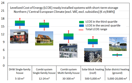
Chart: Task 52 / Technology and Demonstrators study
“Cost analysis on the basis of levelised cost of energy is a widespread method to compare different energy generation technologies. The idea behind this approach is to compare the total costs (= fixed + variable ones) in reference to an energy supply system with the energy supplied by this system over its lifetime,” Mauthner explained. “In the framework of IEA SHC Task 52, I calculated the levelised cost of heat generated by different solar thermal applications and typical system sizes – from small residential systems to large plants connected to heating networks. The calculated levelised cost, expressed in euro cents per kilowatt hour, indicate a price range for heat generated by solar thermal. The estimated range remained constant over the lifetime of the system for each application which was investigated.” In the Task 52 study, Mauthner applied the method based on the research document A review of solar photovoltaic levelised cost of electricity, which was published jointly by Queen´s University in Canada and Michigan Technological University in the USA in 2011 (see the link below). Mauthner added: “In 2013, German Fraunhofer ISE published a study containing a similar approach.”
The economic model which was used for the Task 52 study treats LCOE as the constant unit cost (per kWh) of a payment stream which has the same present value as the total cost incurred by installing and operating the energy-producing installation over its lifetime. The LCOE figures are calculated by adding up the investment and the discounted O&M costs and dividing the total by the solar yield as well discounted over the system’s lifetime (see formula on page 5 of the attached Task 52 study). In this model, the net present value – the difference between positive and negative cash flows – is zero and the discount rate is equal to the return of investment.
Five parameters impact LCOE results
“LCOE calculations are difficult, since the external data required and the assumptions to be made have a great impact on results.” According to the author, five parameters exert a key influence on LCOE calculations (ranked by level of impact on the result):
- Investment
- Service life of system
- Discount rate
- Solar yields
- Operation and maintenance (O&M
Investment
The investment adds onto the initial material costs of the system and the labour costs for installation. The first factor is based on what costs can be clearly attributed to the solar thermal system. In the Task 52 study, Mauthner considered the collector field, its pipework and the entire storage tank and control system to be part of the investment. The range of system plus installation costs in EUR/m2gross was derived from a set of best-practice examples, which had been in operation in countries participating in IEA SHC Task 52 (see also an earlier news piece link to http://www.solarthermalworld.org/content/iea-shc-task-52-seeking-cost-optimised-urban-energy-systems). Another thing that needed to be specified in concrete terms was the cost data: In the Task 52 study, all cost data referred to end-user (customer) prices, but excluded VAT or subsidies.
Service life of the system
The Europe-focused Task 52 study assumes a lifetime of 25 years for all considered pumped system types. However, Mauthner emphasised that there were different lifetime expectations for pumped systems outside Europe. For example, China shows 15 years for pumped systems and ten for thermosiphon systems. The service life estimate is a highly sensitive parameter, which significantly influences the LCOE (longer service life consequently results in lower LCOE).
Discount rate / internal rate of return
As described above, the LCOE calculations are based on the net present value method, in which all cash inflow/outflow over the lifetime of an asset is discounted back to a common reference date, usually to its present value. The determination of the discount rate has a strong impact on results and describes the internal rate of return. Mauthner’s calculations were based on two principal assumptions: He assumed that the minimal intended internal rate of return was 3 % and he disregarded inflation rates by using a nominal discount rate. “Obviously, commercial clients will expect a higher IRR rate than 3 %, which would increase the LCOE, but the technological comparison was at the heart of the Task 52 benchmark study,” Mauthner explained his approach. His method, including all of the benchmark figures and assumptions he made, can be adapted to different customer case studies by changing the discount rate. The above-mentioned study by Fraunhofer ISE for example used the weighted average cost of capital (WACC) to determine the discount rate and considers the usual cost of capital on the market.
Solar yields
The most important assumption here again points to the boundaries of the system, for example, if the solar yield is measured in front of or behind the storage tank. Mauthner referred to annually delivered, specific useful solar thermal energy per gross collector area in kWh/m²gross·a, considering thermal losses in the solar loop pipework and the thermal energy storage.
“In the Task 52 study, we used metered useful energy yields as much as possible, or optionally T-Sol program simulations for the climate in question. It is important to know whether the specified collector array refers to gross or aperture area,” Mauthner explained. “This kind of inaccuracy results in considerable error margins, especially with regard to vacuum tube collectors, where they add up to around 50 %, while flat plate panels have around 10 %.”
Operation and maintenance (O&M)
O&M costs for solar thermal systems are rather small and have the least impact on LCOE results. Mauthner differentiates between fixed operating costs for service, maintenance, repairs and insurance, and variable ones like electricity demand for pumps. Based on the experiences gained with systems that had already been in operation, the fixed operating costs of small systems were set at 1 % of the investment, excluding labour, and at 0.75 % for large installations. Mauthner gave variable operating expenses the common benchmark value of 0.015 kWhel per kWhth, which was confirmed by on-site metering of solar thermal installations (average COP = 69). However, large systems like the solar district heating plants in Denmark will go below the above-mentioned O&M cost assumptions, which is why these numbers are typically used for smaller systems.
The following table shows an overview of the assumptions which formed the basis of the LCOE calculations also shown in the chart above.
|
ST system category
|
Domestic hot water system in single-family home
|
Combi system in single-family home
|
Combi system in multi-family building
|
Solar-assisted block heating system
|
Solar district heating system
|
|
Installation
|
On roof
|
On roof
|
On roof
|
On roof
|
At ground level
|
|
Common size [m²]
|
5–10 m²
|
12–24 m²
|
30–300 m²
|
500–5,000 m²
|
5,000–20,000 m²
|
|
Typical short-term storage
|
Domestic hot water tank
|
Pressurised thermal energy storage
|
Pressurised thermal energy storage
|
Pressurised thermal energy storage
|
Non- pressurised thermal energy storage
|
|
Investment I0 [€/m²gross]
|
810 – 1,050
|
670 – 860
|
520 – 790
|
420 – 660
|
210 – 270
|
|
Useful energy yield SE [kWh/m²gross]
|
380
|
330
|
400
|
390
|
410
|
|
Fixed and variable O&M costs [€/m²gross]
|
0.008
|
0.007
|
0.007
|
0.005
|
0.003
|
|
Discount rate
|
3 %
|
3 %
|
3 %
|
3 %
|
3 %
|
|
Service life [a]
|
25
|
25
|
25
|
25
|
25
|
|
LCOE [EUR cent/kWh]
|
14.3 – 18.1
|
13.7 – 17.4
|
8.9 – 13.4
|
7.3 – 11.2
|
3.7 – 4.6
|
Benchmark figures and assumptions to calculate the LCOE in northern / central Europe for selected applications. The heat cost range was derived from the range of investment amounts. This LCOE calculation model does not consider financing or inflation, nor the degradation of collector efficiency or any residual value of the asset.
Source: Task 52 study
Websites of institution and projects mentioned in the article:
A review of solar photovoltaic levelised cost of electricity: http://www.sciencedirect.com/science/article/pii/S1364032111003492